<?xml version="1.0" encoding="utf-8"?><feed xmlns="http://www.w3.org/2005/Atom" ><generator uri="https://jekyllrb.com/" version="3.10.0">Jekyll</generator><link href="/feed.xml" rel="self" type="application/atom+xml" /><link href="/" rel="alternate" type="text/html" /><updated>2026-03-16T01:55:16+00:00</updated><id>/feed.xml</id><title type="html">Your awesome title</title><subtitle>Write an awesome description for your new site here. You can edit this line in _config.yml. It will appear in your document head meta (for Google search results) and in your feed.xml site description.</subtitle><entry><title type="html">🇻🇳 Hải Vân Pass, Vietnam</title><link href="/hai_van_pass/" rel="alternate" type="text/html" title="🇻🇳 Hải Vân Pass, Vietnam" /><published>2026-02-24T08:00:00+00:00</published><updated>2026-02-24T08:00:00+00:00</updated><id>/hai_van_pass</id><content type="html" xml:base="/hai_van_pass/"><![CDATA[<hr />

<p><img src="../images/hai_van_pass/da_nang.png" alt="da_nang" class="float-right" /></p>

<table class="responsive-table">
  <tbody>
    <tr>
      <td><span style="font-size: 16px;"> 🚴: <a href="https://www.strava.com/activities/17336089926" target="_blank">Strava</a> 🎧: <a href="https://youtu.be/mfU825Pg9k8?t=3389" target="_blank">Coulou</a> </span></td>
    </tr>
  </tbody>
</table>

<table class="about_table">
  <tbody>
    <tr>
      <td><span style="font-size: 1px;"> . </span></td>
    </tr>
  </tbody>
</table>

<hr />

<table class="about_table">
  <tbody>
    <tr>
      <td><span style="font-size: 1px;"> . </span></td>
    </tr>
  </tbody>
</table>]]></content><author><name>Sergey Ostrikov</name></author><summary type="html"><![CDATA[]]></summary></entry><entry><title type="html">🇯🇵 Naha, Nago, Okinawa</title><link href="/naha_nago_okinawa/" rel="alternate" type="text/html" title="🇯🇵 Naha, Nago, Okinawa" /><published>2026-02-24T08:00:00+00:00</published><updated>2026-02-24T08:00:00+00:00</updated><id>/naha_nago_okinawa</id><content type="html" xml:base="/naha_nago_okinawa/"><![CDATA[<hr />

<p><img src="../images/naha_nago_okinawa/okinawa.png" alt="okinawa" class="float-right" /></p>

<table class="responsive-table">
  <tbody>
    <tr>
      <td><span style="font-size: 16px;"> 🚴: <a href="https://www.strava.com/activities/16861918300" target="_blank">Strava</a> 🎧: <a href="https://youtu.be/mfU825Pg9k8?t=3389" target="_blank">Coulou</a> </span></td>
    </tr>
  </tbody>
</table>

<table class="responsive-table">
  <tbody>
    <tr>
      <td><span style="font-size: 16px;"> 
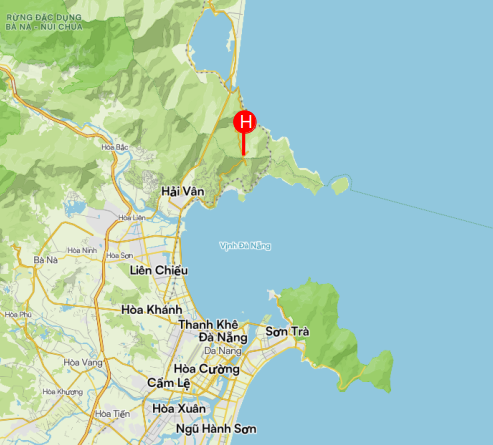
Boxy cars passing on the right, chain spinning, legs waking up: good morning Okinawa! </span></td>
    </tr>
    <tr>
      <td><span style="font-size: 16px;"> Staying on the left side of the road is foreign to me. Not only do I have to look over my right shoulder, I also have to be mindful of turns: left - roll, right - stop. My instincts are useless. But somehow it’s not constraining. Okinawa is chill like that. </span></td>
    </tr>
    <tr>
      <td><span style="font-size: 16px;"> 
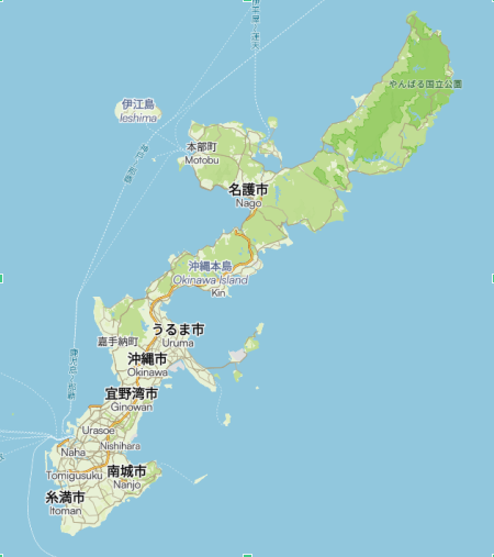
Japan is smaller than California. Slightly larger than Germany. Okinawa is one of 426 inhabited islands in the area. And there are anywhere between 3000 and 6852 islands south of the main island. I know that from a book on the <a href="https://www.amazon.com/Okinawa-Ryukyu-Islands-Comprehensive-Entire/dp/4805312335" target="_blank">Ryukyu Islands</a> I was just reading, which was weirdly inspiring. It reminded me of another book: Ostrov Sakhalin. Dry and filled with stats, yet it just flows. </span></td>
    </tr>
  </tbody>
</table>

<hr />

<table class="responsive-table">
  <tbody>
    <tr>
      <td><span style="font-size: 16px;"> Something to think about, some pedaling to do, Pocari Sweat in my water bottle, it doesn’t get better than this. I’m headed up north until I feel it’s time to turn back. У самурая нет цели, только путь. </span></td>
    </tr>
  </tbody>
</table>

<table class="responsive-table">
  <tbody>
    <tr>
      <td><span style="font-size: 45px;"> WIP </span></td>
    </tr>
  </tbody>
</table>

<table class="about_table">
  <tbody>
    <tr>
      <td><span style="font-size: 1px;"> . </span></td>
    </tr>
  </tbody>
</table>

<hr />

<table class="about_table">
  <tbody>
    <tr>
      <td><span style="font-size: 1px;"> . </span></td>
    </tr>
  </tbody>
</table>]]></content><author><name>Sergey Ostrikov</name></author><summary type="html"><![CDATA[]]></summary></entry><entry><title type="html">🇺🇸 Oahu, Hawaii</title><link href="/oahu_hawaii/" rel="alternate" type="text/html" title="🇺🇸 Oahu, Hawaii" /><published>2026-02-24T08:00:00+00:00</published><updated>2026-02-24T08:00:00+00:00</updated><id>/oahu_hawaii</id><content type="html" xml:base="/oahu_hawaii/"><![CDATA[<hr />

<p><img src="../images/oahu_hawaii/oahu.png" alt="oahu" class="float-right" /></p>

<table class="responsive-table">
  <tbody>
    <tr>
      <td><span style="font-size: 16px;"> 🚴: <a href="https://www.strava.com/activities/5310278187" target="_blank">Strava</a> 🎧: <a href="https://youtu.be/mfU825Pg9k8?t=3389" target="_blank">Coulou</a> </span></td>
    </tr>
  </tbody>
</table>

<table class="about_table">
  <tbody>
    <tr>
      <td><span style="font-size: 1px;"> . </span></td>
    </tr>
  </tbody>
</table>

<hr />

<table class="about_table">
  <tbody>
    <tr>
      <td><span style="font-size: 1px;"> . </span></td>
    </tr>
  </tbody>
</table>]]></content><author><name>Sergey Ostrikov</name></author><summary type="html"><![CDATA[]]></summary></entry><entry><title type="html">🇹🇼 Wuling Pass (雲海)</title><link href="/wuling_pass/" rel="alternate" type="text/html" title="🇹🇼 Wuling Pass (雲海)" /><published>2026-02-21T08:00:00+00:00</published><updated>2026-02-21T08:00:00+00:00</updated><id>/wuling_pass</id><content type="html" xml:base="/wuling_pass/"><![CDATA[<hr />

<p><img src="../images/wuling_pass/train.gif" alt="train" class="float-right" /></p>

<table class="responsive-table">
  <tbody>
    <tr>
      <td><span style="font-size: 16px;"> 🚴: <a href="https://www.strava.com/activities/16808112054" target="_blank">Strava</a> 🎧: <a href="https://youtu.be/mfU825Pg9k8?t=3389" target="_blank">Coulou</a> </span></td>
    </tr>
  </tbody>
</table>

<table class="responsive-table">
  <tbody>
    <tr>
      <td><span style="font-size: 16px;"> 
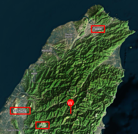
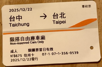
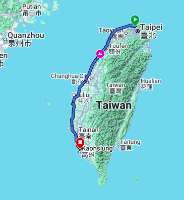
Taiwan is the land of trains. Railway abbreviations weave their way into your vocabulary: MRT for trips within Taipei, TR and HSR for the cities beyond. But it’s also an island of mountain peaks the trains can’t reach. Resting on its way to Taichung, my bike doesn’t know what’s coming. But I do. The highest paved road on the island… </span></td>
    </tr>
  </tbody>
</table>

<hr />

<table class="responsive-table">
  <tbody>
    <tr>
      <td><span style="font-size: 16px;"> Not. So. Fast. Cow. Boy. Ten minutes into the ride, my water bottle bounces into the bushes. I hop off my bike to look for it and find I’ve got a flat, too. </span></td>
    </tr>
  </tbody>
</table>

<table class="responsive-table">
  <tbody>
    <tr>
      <td><span style="font-size: 16px;"> A few minutes later, a local cyclist I’d bumped into at the train station hands me my water bottle. “Man, I don’t know you, but you look a bit underprepared to go out alone at night. It’s cold up there. No gloves? Your hands will freeze. You won’t be able to brake on the way down. I got a car. Let me take you to Puli. It’s a better starting point.” </span></td>
    </tr>
  </tbody>
</table>

<hr />

<p><img src="../images/wuling_pass/wuling.png" alt="wuling" class="float-left" /></p>

<table class="responsive-table">
  <tbody>
    <tr>
      <td><span style="font-size: 16px;"> 
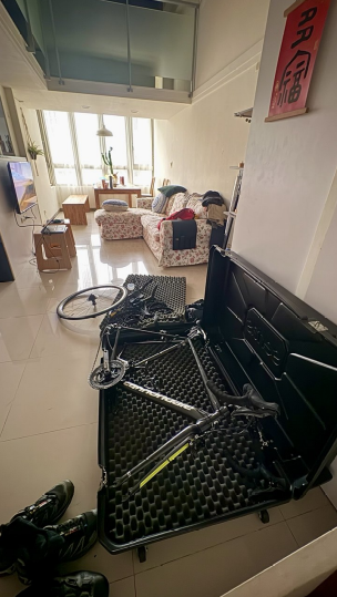
I slide the wheel back into the rear dropouts, insert the skewer, tighten the lever, and glance at my phone: 1 AM. This whole thing is starting to feel forced. I dragged myself out of bed, took two trains, circled the station struggling to find a way out, and now I’m fixing a flat with my hands all greasy. I agree, slightly <a href="https://www.strava.com/activities/16805082962" target="_blank">deflated</a>. </span></td>
    </tr>
  </tbody>
</table>

<hr />

<table class="responsive-table">
  <tbody>
    <tr>
      <td><span style="font-size: 16px;"> Jokes aside, a big shout-out to <a href="https://www.instagram.com/jasonchijuchiang/" target="_blank"><strong>Jason</strong></a> for saving the day! <span style="font-size: 22px;"> 🙌 </span> </span></td>
    </tr>
  </tbody>
</table>

<hr />

<p><img src="../images/wuling_pass/puli_night.gif" alt="puli_night" class="float-right" /></p>

<hr />

<table class="responsive-table">
  <tbody>
    <tr>
      <td><span style="font-size: 16px;"> Next thing I know I’m in Puli, a small town at the foot of a mountain range. It’s dead quiet at 3 AM. This is my new start. Yeehaw! </span></td>
    </tr>
  </tbody>
</table>

<hr />

<table class="responsive-table">
  <tbody>
    <tr>
      <td><span style="font-size: 16px;"> Not. So. Fast. Cow. Boy. Gotta wash my hands first. That out of the way, ahead of me is a sloooooooooow grind: 25 miles with a 6.5% average grade. Takes me five hours to reach Wuling Pass. But here it is: the sea of clouds (雲海). And the frost on the handrail. Frost in Taiwan… Who would’ve thought? </span></td>
    </tr>
  </tbody>
</table>

<hr />

<p><img src="../images/wuling_pass/sea_of_clouds.gif" alt="sea_of_clouds" class="float-left" />
<img src="../images/wuling_pass/frost.png" alt="frost" class="float-left" /></p>

<p><img src="../images/wuling_pass/3275.png" alt="3275" class="float-left" /></p>

<table class="responsive-table">
  <tbody>
    <tr>
      <td><span style="font-size: 16px;"> 
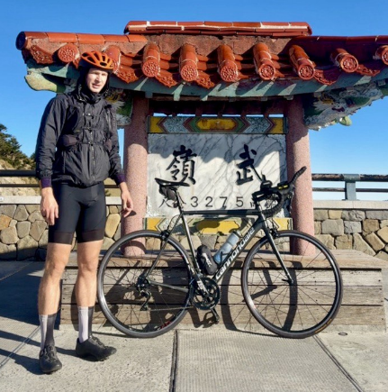
Concerned about turning into a popsicle on the way down, I pull two pairs of plastic food-handling gloves from my pocket. I got them at 7-Eleven, along with two rubber bands to keep the cold air out. I was warned, so, I prepped a bit to <a href="https://en.wikipedia.org/wiki/Roll_Safe" target="_blank">Roll Safe</a>, or warm, at least. </span></td>
    </tr>
    <tr>
      <td><span style="font-size: 16px;"> Climbing is fun. Rolling downhill for 70 miles? Terrifying. It is too steep and cold to have my phone out. Such a shame I don’t have my GoPro with me either, because the 30-mile ride down to Puli is a visual journey. </span></td>
    </tr>
    <tr>
      <td><span style="font-size: 16px;"> Back in Puli, safe, I peel off my windbreaker. The air is warmer, the ground flatter. Feels strange to be back. It was a different world just a few hours ago. The final 40 miles are a slight downhill to Taichung. A gradual return to civilization. More lights, more traffic, and trains… again. </span></td>
    </tr>
  </tbody>
</table>

<hr />

<p><img src="../images/wuling_pass/hsr.png" alt="hsr" class="float-right" /></p>

<table class="responsive-table">
  <tbody>
    <tr>
      <td><span style="font-size: 16px;"> I hop on the HSR, and I’m back in Taipei. The main station is hella busy in the evening. The subway cars are packed. A bit surprised but understanding, people make space for my bike, and the red MRT line takes me all the way up to Zhongyi, where my journey began. It’s a long ride, some 14 stops. Somehow it feels even longer than the climb. But this is it: I step out of the station and reassemble my bike for the last mile back to my Airbnb. Goodbye trains. Goodbye, Taiwan. </span></td>
    </tr>
  </tbody>
</table>

<table class="responsive-table">
  <tbody>
    <tr>
      <td><span style="font-size: 16px;"> Goodbye for now. </span></td>
    </tr>
  </tbody>
</table>

<hr />

<p><img src="../images/wuling_pass/mrt.gif" alt="mrt" class="float-left" /></p>

<p><img src="../images/wuling_pass/airbnb.png" alt="airbnb" class="float-left" /></p>

<table class="about_table">
  <tbody>
    <tr>
      <td><span style="font-size: 1px;"> . </span></td>
    </tr>
  </tbody>
</table>

<hr />

<table class="about_table">
  <tbody>
    <tr>
      <td><span style="font-size: 1px;"> . </span></td>
    </tr>
  </tbody>
</table>]]></content><author><name>Sergey Ostrikov</name></author><summary type="html"><![CDATA[]]></summary></entry><entry><title type="html">🇹🇼 Taipei → Kaohsiung</title><link href="/taipei_kaohsiung/" rel="alternate" type="text/html" title="🇹🇼 Taipei → Kaohsiung" /><published>2026-02-20T08:00:00+00:00</published><updated>2026-02-20T08:00:00+00:00</updated><id>/taipei_kaohsiung</id><content type="html" xml:base="/taipei_kaohsiung/"><![CDATA[<hr />

<p><img src="../images/taipei_kaohsiung/cycling_taiwan.png" alt="cycling_taiwan" class="float-right" /></p>

<table class="responsive-table">
  <tbody>
    <tr>
      <td><span style="font-size: 16px;"> 🚴: <a href="https://www.strava.com/activities/16727548624" target="_blank">Strava</a> 🎧: <a href="https://youtu.be/mfU825Pg9k8?t=3389" target="_blank">Coulou</a> </span></td>
    </tr>
    <tr>
      <td><span style="font-size: 16px;"> Empty streets, foreign country, tailwind: my trusty Cannondale and I are soaring. This is a night ride.  </span></td>
    </tr>
    <tr>
      <td><span style="font-size: 16px;"> I left Taipei at 10 PM. </span></td>
    </tr>
    <tr>
      <td><span style="font-size: 16px;"> Up close: the hum of my tires, the whir of the chain, and the warm, balmy air rushing past. From afar: a tiny, throbbing light travelling through the vast darkness, loosely following <a href="https://en.wikipedia.org/wiki/Taiwan_Cycling_Route_No.1" target="_blank">環島1號線</a>, Taiwan’s Cycling Route #1. </span></td>
    </tr>
    <tr>
      <td><span style="font-size: 16px;"> Past midnight, a 7-Eleven glows ahead like a lighthouse. I glide in, still buzzing. The clerk nods. I grab onigiri and a local electrolyte drink. They give me exactly the kind of boost my body needs, and I roll back into the dark. </span></td>
    </tr>
  </tbody>
</table>

<hr />

<p><img src="../images/taipei_kaohsiung/video_note.gif" alt="video_note" class="float-left" /></p>

<table class="responsive-table">
  <tbody>
    <tr>
      <td><span style="font-size: 16px;"> The landscape is a mystery of dark shapes: rice paddies, I think, and low industrial buildings. I’m not exactly a tourist seeing sights; more of a ghost passing through, connected to the island by this thin strip of road. </span></td>
    </tr>
    <tr>
      <td><span style="font-size: 16px;"> Convenience stores! These little oases of light become my only landmarks. At the next one, I report to a couple of my buddies on Telegram: I’m at mile 80, somewhere in Taiwan, feeling great. Phone’s internet is sluggish. Takes a couple minutes for the video note to go out, but I’m not sweating it. I got me a lemon cake and milk tea this time. </span></td>
    </tr>
  </tbody>
</table>

<hr />

<p><img src="../images/taipei_kaohsiung/lukang.png" alt="lukang" class="float-right" /></p>

<table class="responsive-table">
  <tbody>
    <tr>
      <td><span style="font-size: 16px;"> 
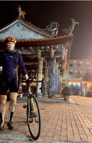
Past 100mi the ride no longer feels like soaring, but also far from grinding. Rolling through a town asleep, I hear how loud the spring-loaded pawls become, rapidly snapping into the ratchet teeth. <strong>CLICK, CLICK, CLICK, CLICK, CLICK, CLICK, click, click, click, click, click, click, click, click, click, click</strong>, click, click, click, click, click, click, click, click, click, click, click. I catch myself pedaling quieter, marveling at an old temple, its weathered grace. Pressing the brakes, I unclip into complete silence. This is my halfway point. Another town I’ll never know by daylight. Not in this way. </span></td>
    </tr>
  </tbody>
</table>

<hr />

<table class="about_table55r">
  <tbody>
    <tr>
      <td><span style="font-size: 16px;"> Облегчённо вздыхают одни <br /> Друзья говорят - “устал” <br /> Ошибаются те и другие <br /> - это привал… </span></td>
    </tr>
  </tbody>
</table>

<table class="about_table">
  <tbody>
    <tr>
      <td><span style="font-size: 16px;">  </span></td>
    </tr>
  </tbody>
</table>

<p><img src="../images/taipei_kaohsiung/sunrise.gif" alt="sunrise" class="float-left" /></p>

<hr />

<table class="responsive-table">
  <tbody>
    <tr>
      <td><span style="font-size: 16px;"> The second half is bound to be a battle against the heat. </span></td>
    </tr>
    <tr>
      <td><span style="font-size: 16px;"> At sunrise, Garmin reads 130mi and my body reads hungry. Let the sun climb, but I need a full breakfast. <strong>My Warm Day</strong> cafe (<a href="https://www.google.com/maps/@23.7957001,120.2798343,3a,79y,357.44h,124.71t/data=!3m7!1e1!3m5!1sb7URJaWQxitK4jDrhh5C7Q!2e0!6shttps:%2F%2Fstreetviewpixels-pa.googleapis.com%2Fv1%2Fthumbnail%3Fcb_client%3Dmaps_sv.tactile%26w%3D900%26h%3D600%26pitch%3D-34.714625092703244%26panoid%3Db7URJaWQxitK4jDrhh5C7Q%26yaw%3D357.4363364328135!7i16384!8i8192?entry=ttu&amp;g_ep=EgoyMDI2MDIxNy4wIKXMDSoASAFQAw%3D%3D" target="_blank">麥味登</a>), next to Fried Chicken Master, looks like it’d take Apple Pay. </span></td>
    </tr>
    <tr>
      <td><span style="font-size: 16px;"> I pop in. The girls are giggling. I realize I’m a spectacle with my orange helmet on. I point to noodles with black pepper sauce, chicken, and soy milk. The food is here. Gotta log it. The Oura app says: high in protein, carbs &amp; fats, low in fiber, and moderate in processing level &amp; added sugars. Classifies it as barely nutritious. I classify it as great! </span></td>
    </tr>
  </tbody>
</table>

<p><img src="../images/taipei_kaohsiung/200mi.png" alt="200mi" class="float-right" /></p>

<hr />

<table class="responsive-table">
  <tbody>
    <tr>
      <td><span style="font-size: 16px;"> 
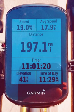
Almost 200mi in, the heat is a physical force. My legs are getting heavy, my nose sunburnt, but I can fool my senses for a little while: I pretend I’m racing the cars beside me. I glide past them, and for a moment I’m winning. Every dog has its day. They are not racing, of course. Just commuting, running errands, hauling. The road does not care, it takes us all. Mine is just this sweet illusion, helping me battle the heat. </span></td>
    </tr>
  </tbody>
</table>

<hr />

<p><img src="../images/taipei_kaohsiung/tainan.gif" alt="tainan" class="float-left" />
<img src="../images/taipei_kaohsiung/stoplights.gif" alt="stoplights" class="float-left" /></p>

<table class="about_table38">
  <tbody>
    <tr>
      <td><span style="font-size: 16px;"> The last 28mi cross into Kaohsiung, toward a train station. The roads get busier and things slow to a crawl. Feeling accomplished, I don’t resist the stop &amp; go as much. This is my island etude: playing it slow, playing it long, playing it home. </span></td>
    </tr>
  </tbody>
</table>

<hr />

<table class="about_table38">
  <tbody>
    <tr>
      <td><span style="font-size: 16px;"> The train swallows me, my bike, and 225 miles of road. Two hours later, I’m back in Taipei. Beitou hot springs remind my legs they are just legs. Soaring is over. What’s left is the quiet throb of having experienced it. </span></td>
    </tr>
  </tbody>
</table>

<table class="about_table">
  <tbody>
    <tr>
      <td><span style="font-size: 1px;"> . </span></td>
    </tr>
  </tbody>
</table>

<hr />

<table class="about_table">
  <tbody>
    <tr>
      <td><span style="font-size: 1px;"> . </span></td>
    </tr>
  </tbody>
</table>]]></content><author><name>Sergey Ostrikov</name></author><summary type="html"><![CDATA[]]></summary></entry><entry><title type="html">Analog Inference</title><link href="/analog_inference/" rel="alternate" type="text/html" title="Analog Inference" /><published>2026-02-15T08:00:00+00:00</published><updated>2026-02-15T08:00:00+00:00</updated><id>/analog_inference</id><content type="html" xml:base="/analog_inference/"><![CDATA[<hr />

<p><img src="../images/analog_inference/sf_ride_seg.gif" alt="sf_ride_seg" class="center_gif" /></p>

<hr />

<table class="responsive-table">
  <tbody>
    <tr>
      <td><span style="font-size: 16px;"> For workloads executing on analog compute fabrics, power can be slashed by orders of magnitude at the expense of computational accuracy. While this tradeoff offers clear power benefits, inherent circuit noise introduces variability into computational results, making accuracy evaluation a nuanced statistical exercise. </span></td>
    </tr>
    <tr>
      <td><span style="font-size: 16px;"> This page describes an evaluation approach that tracks <strong>the effects of circuit noise</strong> on image segmentation models, whose primary tasks are <strong>object localization</strong> and <strong>classification</strong>. Extending the <a href="https://en.wikipedia.org/wiki/Evaluation_measures_(information_retrieval)#Average_precision" target="_blank">average precision</a> metric (AP), this approach captures and quantifies the impact of noise on both of these tasks. </span></td>
    </tr>
    <tr>
      <td><span style="font-size: 16px;"> In a standard evaluation, detections (DT) are compared against ground truths (GT) from a validation dataset. At its core, this is a traditional binary classification process with four (true/false positive/negative) outcomes:  </span></td>
    </tr>
  </tbody>
</table>

\[\begin{array}{c|cc}
&amp; \text{DT: } 1 &amp; \text{DT: } 0 \\ \hline
\text{GT: } 1 &amp; \text{TP ↑} &amp; \text{FN ↓} \\
\text{GT: } 0 &amp; \text{FP ↓} &amp; \text{TN ↑}
\end{array}\]

<table class="responsive-table">
  <tbody>
    <tr>
      <td><span style="font-size: 16px;"> Add noise, and this process gets trickier: outcomes become variable. This means that some detections may travel across the TP, FP, FN, TN categories due to noise. This variability is not captured by AP. And while the practical impact may vary, capturing and quantifying such dynamics is essential. </span></td>
    </tr>
  </tbody>
</table>

<hr />

<table class="responsive-table">
  <tbody>
    <tr>
      <td><span style="font-size: 22px;"> Warm-Up Calculation of AP 🐕‍🦺🦮🐩🐕🐶 </span></td>
    </tr>
  </tbody>
</table>

<table class="responsive-table">
  <tbody>
    <tr>
      <td><span style="font-size: 16px;"> Let’s say there’s a total of 50 dogs in the entire validation dataset spread across 100 images. Naturally, a trained model would generate low scores for images with no dogs, high scores for images with dogs, and medium scores for images with similar-looking animals. </span></td>
    </tr>
    <tr>
      <td><span style="font-size: 16px;"> The plot below represents a typical evaluation run with two distinct but overlapping distributions. The scores range from <span style="font-size: 16px; color: #a82a2a; "> <strong>0.00 to 0.60</strong> </span> for <span style="font-size: 16px; color: #a82a2a; "> <strong>no dogs</strong></span> and from <span style="font-size: 16px;  color: #2b31fb; "> <strong>0.35 to 1.00</strong></span> for <span style="font-size: 16px;  color: #2b31fb; "> <strong>dogs</strong></span>. For a comprehensive evaluation, the scores are classified using multiple thresholds rather than a single one. And even though the middle region is where the action takes place, classification is performed across the entire scale, from far left to far right. </span></td>
    </tr>
  </tbody>
</table>

<table class="responsive-table">
  <tbody>
    <tr>
      <td><span style="font-size: 1px;"> . </span></td>
    </tr>
  </tbody>
</table>

<p><img src="../images/analog_inference/dogs_no_dogs.gif" alt="dogs_no_dogs" class="center_gif" /></p>

<table class="responsive-table">
  <tbody>
    <tr>
      <td><span style="font-size: 1px;"> . </span></td>
    </tr>
  </tbody>
</table>

<table class="responsive-table">
  <tbody>
    <tr>
      <td><span style="font-size: 16px;"> To provide a concise numerical example, I make up predictions, cluster them at 10 confidence scores, and couple with an intersection over union (IoU) level in the table below (left). This allows a full sweep of the scale with only 11 evaluation thresholds, resulting in 11 binary classifications (right). Each classification yields a (TP, FP, FN, TN) set and is reduced to recall \((R)\) and precision \((P)\) ratios. The 11 precision ratios are further condensed into a single \(AP\) value using an appropriate <strong>measure of central tendency (MoT)</strong>. This process is performed across 10 IoU thresholds resulting in 10 \(AP_{dog\ @\ IoU}\) values which are then averaged to get the final \(AP_{dog} = \frac{1}{10} \sum AP_{dog\ @\ IoU}\). </span></td>
    </tr>
    <tr>
      <td><span style="font-size: 1px;"> . </span></td>
    </tr>
  </tbody>
</table>

\[\begin{array}{c|cc}
\text{score} &amp; \text{dogs} &amp; \text{no dogs} &amp; \text{IoU} \\ \hline
\text{0.95} &amp; \text{1} &amp; \text{0} &amp; 0.85 \\
\text{0.85} &amp; \text{3} &amp; \text{0} &amp; 0.80 \\
\text{0.75} &amp; \text{10} &amp; \text{0} &amp; 0.75 \\
\text{0.65} &amp; \text{25} &amp; \text{0} &amp; 0.70 \\
\text{0.55} &amp; \text{8} &amp; \text{1} &amp; 0.65 \\
\text{0.45} &amp; \text{2} &amp; \text{4} &amp; 0.60 \\
\text{0.35} &amp; \text{1} &amp; \text{17} &amp; 0.55 \\
\text{0.25} &amp; \text{0} &amp; \text{23} &amp; 0.55 \\
\text{0.15} &amp; \text{0} &amp; \text{4} &amp; 0.55 \\
\text{0.05} &amp; \text{0} &amp; \text{1} &amp; 0.55 \\
\end{array}
\qquad
\begin{array}{c|cc}
\text{threshold} &amp; TP &amp; FP &amp; FN &amp; TN &amp; R_{i} &amp; P_{i} &amp; {i} \\ \hline
\text{1.00} &amp; 0  &amp; 0  &amp; 50 &amp; 50 &amp; 0.00 &amp; 1.00 &amp; 1 \\
\text{0.90} &amp; 1  &amp; 0  &amp; 49 &amp; 50 &amp; 0.02 &amp; 1.00 &amp; 2 \\
\text{0.80} &amp; 4  &amp; 0  &amp; 46 &amp; 50 &amp; 0.08 &amp; 1.00 &amp; 3 \\
\text{0.70} &amp; 14 &amp; 0  &amp; 36 &amp; 50 &amp; 0.28 &amp; 1.00 &amp; 4 \\
\text{0.60} &amp; 39 &amp; 0  &amp; 11 &amp; 50 &amp; 0.78 &amp; 1.00 &amp; 5 \\
\text{0.50} &amp; 47 &amp; 1  &amp; 3  &amp; 49 &amp; 0.94 &amp; 0.98 &amp; 6 \\
\text{0.40} &amp; 49 &amp; 5  &amp; 1  &amp; 45 &amp; 0.98 &amp; 0.91 &amp; 7 \\
\text{0.30} &amp; 50 &amp; 22 &amp; 0  &amp; 28 &amp; 1.00 &amp; 0.69 &amp; 8 \\
\text{0.20} &amp; 50 &amp; 45 &amp; 0  &amp; 5  &amp; 1.00 &amp; 0.53 &amp; 9 \\
\text{0.10} &amp; 50 &amp; 49 &amp; 0  &amp; 1  &amp; 1.00 &amp; 0.51 &amp; 10 \\
\text{0.00} &amp; 50 &amp; 50 &amp; 0  &amp; 0  &amp; 1.00 &amp; 0.50 &amp; 11 \\
\end{array}\]

<table class="responsive-table">
  <tbody>
    <tr>
      <td><span style="font-size: 1px;"> . </span></td>
    </tr>
  </tbody>
</table>

<table class="responsive-table">
  <tbody>
    <tr>
      <td><span style="font-size: 16px;"> As a concrete example, I use the MoT below to compute \(AP_{dog}\), where \(P_i\) and \(R_i\) are precision and recall at threshold \(i\) and \(R_{i-1} = 0\). Plugging in the numbers from the table yields 0.987 @ IoU 0.5. And for the sake of completeness, assume that \(AP_{dog,\ IoU}\) drops by 0.100 as IoU threshold tightens \((↑)\) to get the final \(AP_{dog}\). </span></td>
    </tr>
  </tbody>
</table>

\[\text{ (1)}\   AP_{dog\ @\ IoU(0.50)} = \sum_{i=1}^{11} P_i*(R_{i}-R_{i-1}) = 0.987 \\ . \\ . \\ . \\ \text{(10)}\   AP_{dog\ @\ IoU(0.95)} = \sum_{i=1}^{11} P_i*(R_{i}-R_{i-1}) = 0.087\]

<hr />

\[AP_{dog} = \frac{1}{10} \sum_{IoUs} AP_{dog\ @\ IoU} = 0.537\]

<hr />

<table class="responsive-table">
  <tbody>
    <tr>
      <td><span style="font-size: 16px;"> \(AP\) addresses both localization and classification through calculations across IoUs and confidence thresholds, and is deemed sufficient for evaluating image segmentation models. But here comes the noise.</span></td>
    </tr>
  </tbody>
</table>

<hr />

<table class="responsive-table">
  <tbody>
    <tr>
      <td><span style="font-size: 22px;"> Seemingly Good Randomness </span></td>
    </tr>
  </tbody>
</table>

<table class="responsive-table">
  <tbody>
    <tr>
      <td><span style="font-size: 16px;"> Analog computing brings noise into the picture, making computation results inherently variable. This variability originates at the fabric level, affecting fundamental linalg operations like matrix-vector multiplication (MVM), and propagates all the way to confidence score generation. As a result, evaluation becomes more statistical, requiring not only a measure of central tendency but also a <strong>measure of variability (MoV)</strong>. </span></td>
    </tr>
    <tr>
      <td><span style="font-size: 16px;"> Conceptually, a segmentation model can be viewed as a composition of layers with linalg ops. Confidence score generation is therefore a function of the composition of these ops. And since the fundamental ops are noisy, the resulting scores vary as well. Symbolic shorthand: </span></td>
    </tr>
  </tbody>
</table>

\[S = f(img) \qquad → \qquad  f = f_{L} ∘ f_{L−1} ∘ ⋯ ∘ f_{1}\]

\[X_{noise} \sim N(\mu, \sigma^2) \qquad op^{noisy} = op + X_{noise} \qquad → \qquad f_{l}^{noisy} \sim N(op_i + \mu, \sigma^2)\]

\[S = f^{noisy}(img) \qquad → \qquad \tilde{S} \sim D_{pushforward}\]

<table class="responsive-table">
  <tbody>
    <tr>
      <td><span style="font-size: 16px;"> The key is that the score effectively becomes a random variable drawn from a pushforward of the noise distribution through the layers. In other words, for the same input image, each forward pass yields a new realization of the score. Below is a visual representation of this behavior, showing varying scores generated by an analog fabric for the same set of images. </span></td>
    </tr>
  </tbody>
</table>

<p><span style="font-size: 16px; color: #a82a2a; "></span></p>

<p><img src="../images/analog_inference/variable_scores.gif" alt="variable_scores" class="center_gif" /></p>

<table class="responsive-table">
  <tbody>
    <tr>
      <td><span style="font-size: 16px;"> To capture this variability, \(AP_{dog}\) is computed repeatedly over many time points (snapshots of the animation above) and PVT corners, yielding multiple \(APs\). These data points are then treated as any other statistical data: plotted and summarized using appropriate measures of central tendency and variability. </span></td>
    </tr>
    <tr>
      <td><span style="font-size: 16px;"> With standard \(AP\), however, there’s a risk of classifying random outcomes as true positives and true negatives when they happen to match the ground truth. To tease out these seemingly positive effects, I recommend a modification to the traditional classification process: compare noisy detections against a combination of digital detections and ground truths. This refinement makes evaluation more rigorous, <strong>prioritizing average consistency over occasional performance</strong>. </span></td>
    </tr>
  </tbody>
</table>

<table class="responsive-table">
  <tbody>
    <tr>
      <td><span style="font-size: 1px;"> . </span></td>
    </tr>
  </tbody>
</table>

\[\begin{array}{c|cc}
\text{GT} &amp; \text{digital DT} &amp; \text{noisy DT} &amp; \text{classification} &amp; \text{comment} \\ \hline
\ 1 &amp; \text{1} &amp; \text{1} &amp; \text{TP}\\
\ 1 &amp; \text{1} &amp; \text{0} &amp; \text{FN} &amp; \text{anticipated negative effect}\\
\ 1 &amp; \text{0} &amp; \text{1} &amp; \text{TP → FP} &amp; \text{positive but random effect}\\
\ 1 &amp; \text{0} &amp; \text{0} &amp; \text{FN}\\
\ 0 &amp; \text{1} &amp; \text{1} &amp; \text{FP}\\
\ 0 &amp; \text{1} &amp; \text{0} &amp; \text{TN → FN} &amp; \text{positive but random effect}\\
\ 0 &amp; \text{0} &amp; \text{1} &amp; \text{FP} &amp; \text{anticipated negative effect}\\
\ 0 &amp; \text{0} &amp; \text{0} &amp; \text{TN}\\
\end{array}\]

<table class="responsive-table">
  <tbody>
    <tr>
      <td><span style="font-size: 1px;"> . </span></td>
    </tr>
  </tbody>
</table>

<table class="responsive-table">
  <tbody>
    <tr>
      <td><span style="font-size: 16px;"> Together, the modified classification, repeatedly computed \(AP\), and additional MoT and MoV constitute what I simply call <span style="font-size: 16px; color: #a82a2a; "><strong>Analog AP</strong></span>. This metric provides deeper insight than standard \(AP\) for analog computing. </span></td>
    </tr>
  </tbody>
</table>

<hr />

<table class="responsive-table">
  <tbody>
    <tr>
      <td><span style="font-size: 22px;"> Yet, It Is a Summary Statistic </span></td>
    </tr>
  </tbody>
</table>

<table class="responsive-table">
  <tbody>
    <tr>
      <td><span style="font-size: 16px;"> <span style="font-size: 16px; color: #a82a2a; "><strong>Analog AP</strong></span> is a dense metric; some effects may still be buried or averaged out. A sensitivity analysis on individual images or object types can help uncover pain points that <span style="font-size: 16px; color: #a82a2a; "><strong>Analog AP</strong></span> might miss. </span></td>
    </tr>
    <tr>
      <td><span style="font-size: 16px;"> Below is an example of such analysis, sweeping across a noise parameter and tracking the effects. Modeled as a normal distribution, the error caused by noise is added to MVMs performed by the fabric. The animation increases error’s standard deviation from 0.001 to 0.135 and tracks IoUs and confidence scores for two objects: a small, blurry bird on the left and a large, clear bird on the right. </span></td>
    </tr>
  </tbody>
</table>

<table class="responsive-table">
  <tbody>
    <tr>
      <td><span style="font-size: 1px;"> . </span></td>
    </tr>
  </tbody>
</table>

<p><img src="../images/analog_inference/birds_no_birds.gif" alt="birds_no_birds" class="center_gif" /></p>

<table class="responsive-table">
  <tbody>
    <tr>
      <td><span style="font-size: 1px;"> . </span></td>
    </tr>
  </tbody>
</table>

<table class="responsive-table">
  <tbody>
    <tr>
      <td><span style="font-size: 16px;"> The results reveal three key effects of analog noise. First, <strong>object localization is largely unaffected</strong> by higher noise levels: the blue IoUs lines just wobble around their initial levels. Second, <strong>confidence scores decrease</strong> steadily with noise, following a concave-down trajectory. Though, this alone does not cause mispredictions as the confidence drops across other classes as well. And third, objects that are generally harder to detect <strong>(smaller, blurry, overlapping) are more susceptible</strong> to noise, falling below detection thresholds sooner. </span></td>
    </tr>
    <tr>
      <td><span style="font-size: 16px;"> The first two effects are discernible even in the dense metric, but the third one is easily buried due to varying object sizes and overlap conditions. To me, this is a clear sign that looking beyond summary statistics is worthwhile. Together, sensitivity analysis and <span style="font-size: 16px; color: #a82a2a; "><strong>Analog AP</strong></span> can more thoroughly assess end-to-end accuracy, and ultimately help decide on the value of the power-accuracy tradeoff. </span></td>
    </tr>
  </tbody>
</table>

<table class="responsive-table">
  <tbody>
    <tr>
      <td><span style="font-size: 1px;"> . </span></td>
    </tr>
  </tbody>
</table>

<hr />

<table class="responsive-table">
  <tbody>
    <tr>
      <td><span style="font-size: 1px;"> . </span></td>
    </tr>
  </tbody>
</table>]]></content><author><name>Sergey Ostrikov</name></author><summary type="html"><![CDATA[]]></summary></entry><entry><title type="html">Mapping Algorithm for Distributed Computing</title><link href="/mapping_algo/" rel="alternate" type="text/html" title="Mapping Algorithm for Distributed Computing" /><published>2026-01-14T08:00:00+00:00</published><updated>2026-01-14T08:00:00+00:00</updated><id>/mapping_algo</id><content type="html" xml:base="/mapping_algo/"><![CDATA[<hr />

<table class="responsive-table">
  <tbody>
    <tr>
      <td><span style="font-size: 16px;"> For workloads executing on distributed compute fabrics, performance is often limited by data movement rather than computation. As a result, efficient execution depends critically on how the workloads are partitioned and <strong>placed across hardware resources</strong>. </span></td>
    </tr>
    <tr>
      <td><span style="font-size: 16px;"> This page describes an algorithm I developed (<a href="https://github.com/00xnor/mapping_algo" target="_blank"><strong>code</strong></a>) for distributed systems that maps a task graph onto a hardware connectivity graph. The task graph captures computation and communication dependencies, while the hardware graph represents compute elements and their physical interconnects. The algorithm automatically explores a large search space through an iterative process and converges to communication-efficient task assignments while respecting dependency constraints.  </span></td>
    </tr>
    <tr>
      <td><span style="font-size: 16px;"> Based on <a href="https://en.wikipedia.org/wiki/Ant_colony_optimization_algorithms" target="_blank"><strong>Ant Colony Optimization</strong></a>, the algorithm sends out a group of ants to explore possible paths through the hardware graph. Initially, paths are selected randomly, but over iterations selection becomes biased towards more efficient paths. To guide path selection, top-performing ants leave trails where they travel. And to avoid local minima, the trails that aren’t reinforced by top runners gradually fade away. Over time, the system converges on good solutions without exhaustively exploring every possibility. </span></td>
    </tr>
  </tbody>
</table>

<hr />

<p><img src="../images/mapping_algo/linear_mapping.gif" alt="mapping" class="float-right" /></p>

<table class="responsive-table">
  <tbody>
    <tr>
      <td><span style="font-size: 16px;"> The animation <span style="font-size: 20px;"> → </span> features a linear graph being mapped onto a mesh, showing how the algorithm finds one of the <strong>optimal</strong> solutions. Linear graphs are well-suited for developing mapping intuition because the optimal solutions are known. In fact, the mapping for such graphs can be entirely rule-based, following the obvious up/down/left/right/stair/snake patterns. </span></td>
    </tr>
    <tr>
      <td><span style="font-size: 16px;"> However, today’s most prominent workloads are rarely linear. Regardless of what the term <strong>workload</strong> brings to mind, be it hyperscale/orchestration level, multi-agent, neural-network, or micro-op level like decomposition of conv2d into im2col and gemm, it is often a non-linear graph like the one below. Mapping patterns for such graphs aren’t obvious, especially when the mapping space is constrained.
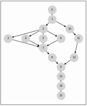
 </span></td>
    </tr>
  </tbody>
</table>

<hr />

<p><img src="../images/mapping_algo/graph.png" alt="mapping" class="float-left" /></p>

<table class="responsive-table">
  <tbody>
    <tr>
      <td><span style="font-size: 16px;"> Consider mapping this <span style="font-size: 20px;"> ← </span> non-linear task graph onto the smallest mesh it can fit into, a 4x4. Having a tight space means that every mapping decision directly impacts subsequent ones. This interdependence makes it challenging to construct a direct solution and apply it generally. </span></td>
    </tr>
    <tr>
      <td><span style="font-size: 32px;  color: #FF5733; "> ———————————— </span></td>
    </tr>
    <tr>
      <td><span style="font-size: 16px;"> More guided than a brute force search, yet not nearly as stringent as a direct solution is the iterative method. It integrates a <strong>heuristic with stochastic elements</strong> to navigate the search space and find satisfactory solutions, including optimal. And sometimes very quickly with proper biasing. But even without nuanced biasing, it’s only a matter of time until a good solution emerges. </span></td>
    </tr>
  </tbody>
</table>

<hr />

<table class="responsive-table">
  <tbody>
    <tr>
      <td><span style="font-size: 22px;">  Give Good Randomness a Chance </span></td>
    </tr>
  </tbody>
</table>

<table class="responsive-table">
  <tbody>
    <tr>
      <td><span style="font-size: 16px;"> The iterative mapping employs <span style="font-size: 16px;  color: #a82a2a; "> <strong>Ants</strong> </span> to search for an optimal path. Each <span style="font-size: 16px;  color: #a82a2a; "> <strong>Ant</strong> </span> starts at a specific location in the hardware graph (e.g. top-left corner in the animation above) and is given a number of choices on where to go next. Before hopping to the next location, the <span style="font-size: 16px;  color: #a82a2a; "> <strong>Ant</strong> </span> assigns a task to the current location and removes it from the task graph marking it as complete. Each <span style="font-size: 16px;  color: #a82a2a; "> <strong>Ant</strong> </span> keeps hopping until all tasks from the task graph are gone. </span></td>
    </tr>
    <tr>
      <td><span style="font-size: 16px;"> This entire process represents an algorithm’s iteration - a single <span style="font-size: 16px;  color: #a82a2a; "> <strong>Ant Colony</strong> </span> run. During the very first run, the <span style="font-size: 16px;  color: #a82a2a; "> <strong>Ants</strong> </span> are unbiased. This means one <span style="font-size: 16px;  color: #a82a2a; "> <strong>randomly</strong> </span> happens to find a more efficient path than the others. Just like in any competition, the winner gets to brag about how it did it: “I started in the top left, moved right, then down…” You get the idea. Having listened to the winner, the next <span style="font-size: 16px;  color: #a82a2a; "> <strong>Ant Colony</strong> </span> run becomes slightly biased towards the <span style="font-size: 16px;  color: #a82a2a; "> <strong>randomly</strong> </span> chosen path. This is good randomness though, as it produced the best result so far. </span></td>
    </tr>
    <tr>
      <td><span style="font-size: 16px;"> To keep producing improvements, the <span style="font-size: 16px;  color: #a82a2a; "> <strong>heuristic</strong> </span> ought to maintain  just the right conditions for randomness to work its magic: providing guidance but also allowing deviaton. Here’s how this is done in practice: </span></td>
    </tr>
    <tr>
      <td><span style="font-size: 16px;">  </span></td>
    </tr>
  </tbody>
</table>

<figure class="highlight"><pre><code class="language-python" data-lang="python"><span class="c1"># Ant's path is constructed by randomly choosing hops.
# Initially, the probabilities are uniformly distributed.
</span><span class="n">choices</span> <span class="o">=</span>       <span class="p">[</span><span class="n">c1</span><span class="p">,</span> <span class="n">c2</span><span class="p">,</span> <span class="p">...,</span> <span class="n">cN</span><span class="p">]</span>
<span class="n">probabilities</span> <span class="o">=</span> <span class="p">[</span><span class="n">p1</span><span class="p">,</span> <span class="n">p2</span><span class="p">,</span> <span class="p">...,</span> <span class="n">pN</span><span class="p">]</span>
<span class="c1"># After normalization:
</span><span class="p">[</span><span class="n">p1</span><span class="p">,</span> <span class="n">p2</span><span class="p">,</span> <span class="p">...,</span> <span class="n">pN</span><span class="p">]</span> <span class="o">=</span> <span class="mi">1</span><span class="o">/</span><span class="n">N</span>

<span class="c1"># After an iteration, hops in the top performer's
# path (e.g., c1, c2) receive a probability boost.
</span><span class="n">choices</span> <span class="o">=</span>       <span class="p">[</span><span class="n">c1</span><span class="p">,</span>     <span class="n">c2</span><span class="p">,</span>     <span class="p">...,</span> <span class="n">cN</span><span class="p">]</span>
<span class="n">probabilities</span> <span class="o">=</span> <span class="p">[</span><span class="n">p1</span> <span class="o">+</span> <span class="n">x</span><span class="p">,</span> <span class="n">p2</span> <span class="o">+</span> <span class="n">x</span><span class="p">,</span> <span class="p">...,</span> <span class="n">pN</span><span class="p">]</span>
<span class="c1"># After normalization:
</span><span class="p">[</span><span class="n">p1</span><span class="p">,</span> <span class="n">p2</span><span class="p">,</span> <span class="p">...,</span> <span class="n">pN</span><span class="p">]</span> <span class="o">=</span> <span class="p">[</span><span class="n">p1</span> <span class="o">+</span> <span class="n">x</span><span class="p">,</span> <span class="n">p2</span> <span class="o">+</span> <span class="n">x</span><span class="p">,</span> <span class="p">...,</span> <span class="n">pN</span><span class="p">]</span><span class="o">/</span><span class="nb">sum</span><span class="p">(</span><span class="n">P</span><span class="p">)</span>

<span class="c1"># Since the first path was chosen randomly,
# the boost shouldn't be excessive.
# A simple model with pheromone deposit and 
# evaporation will do:
</span><span class="n">deposit</span> <span class="o">=</span> <span class="n">AntHeuristicParams</span><span class="p">.</span><span class="n">PHERONOME_DEPOSIT</span>
<span class="n">rate</span> <span class="o">=</span> <span class="n">AntHeuristicParams</span><span class="p">.</span><span class="n">PHERONOME_EVAPORATION_RATE</span>
<span class="n">x</span> <span class="o">=</span> <span class="n">deposit</span> <span class="o">+</span> <span class="p">(</span><span class="mi">1</span> <span class="o">-</span> <span class="n">rate</span><span class="p">)</span><span class="o">*</span><span class="n">current_pheromone</span> 

<span class="c1"># Using deposit = 1.0 and evaporation rate = 0.247:
# The boost for hops in the top performer's path:
</span><span class="n">x</span> <span class="o">=</span> <span class="mf">1.0</span> <span class="o">+</span> <span class="p">(</span><span class="mi">1</span> <span class="o">-</span> <span class="mf">0.247</span><span class="p">)</span><span class="o">*</span><span class="mf">1.0</span> <span class="o">=</span> <span class="mf">1.753</span>
<span class="c1"># The boost for other hops:
</span><span class="n">x</span> <span class="o">=</span> <span class="p">(</span><span class="mi">1</span> <span class="o">-</span> <span class="mf">0.247</span><span class="p">)</span><span class="o">*</span><span class="mf">1.0</span> <span class="o">=</span> <span class="mf">0.753</span>

<span class="c1"># These numbers will translate into probabilities below.
</span>
<span class="c1"># In addition to keeping history of previous choices, 
# path selection is also guided by the energy and time 
# it takes to travel a path. As part of the heuristic, 
# both components depend on the Manhattan distance
# between nodes in the hardware connectivity graph:
</span><span class="n">e_route</span> <span class="o">=</span> <span class="n">AntHeuristicParams</span><span class="p">.</span><span class="n">ENERGY_ROUTE_ONE_BYTE</span>
<span class="n">e_link</span> <span class="o">=</span> <span class="n">AntHeuristicParams</span><span class="p">.</span><span class="n">ENERGY_LINK_ONE_BYTE</span>
<span class="n">energy_per_byte</span> <span class="o">=</span> <span class="p">(</span><span class="n">dist</span> <span class="o">+</span> <span class="mi">1</span><span class="p">)</span><span class="o">*</span><span class="n">e_route</span> <span class="o">+</span> <span class="n">dist</span><span class="o">*</span><span class="n">e_link</span>
<span class="n">n_bytes</span> <span class="o">=</span> <span class="n">dag</span><span class="p">.</span><span class="n">edges</span><span class="p">[</span><span class="n">edge</span><span class="p">][</span><span class="s">'weight'</span><span class="p">]</span>
<span class="n">energy_per_transfer</span> <span class="o">=</span> <span class="n">n_bytes</span><span class="o">*</span><span class="n">energy_per_byte</span>
<span class="n">tau</span> <span class="o">=</span> <span class="mi">1</span><span class="o">/</span><span class="n">energy_per_transfer</span>

<span class="n">t_compute</span> <span class="o">=</span> <span class="n">dag</span><span class="p">.</span><span class="n">nodes</span><span class="p">[</span><span class="n">node</span><span class="p">][</span><span class="s">'weight'</span><span class="p">]</span>
<span class="n">t_communicate</span> <span class="o">=</span> <span class="n">dag</span><span class="p">.</span><span class="n">edges</span><span class="p">[</span><span class="n">edge</span><span class="p">][</span><span class="s">'weight'</span><span class="p">]</span><span class="o">*</span><span class="n">dist</span>
<span class="n">time_total</span> <span class="o">=</span> <span class="n">t_compute</span> <span class="o">+</span> <span class="n">t_communicate</span>
<span class="n">phi</span> <span class="o">=</span> <span class="mi">1</span><span class="o">/</span><span class="n">time_total</span> 

<span class="c1"># Weights alpha and beta adjust the importance of 
# energy and time components respectively:
</span><span class="n">p</span> <span class="o">=</span> <span class="p">(</span><span class="n">tau</span><span class="o">**</span><span class="n">alpha</span><span class="p">)</span><span class="o">*</span><span class="p">(</span><span class="n">phi</span><span class="o">**</span><span class="n">beta</span><span class="p">)</span>

<span class="c1"># Example calculation with dist=3, n_bytes=1024:
# (plugging in 1 femtojoule per byte for communication
# and a 128-bit bus @ 200MHz for communication):
</span><span class="n">n_bytes</span> <span class="o">=</span> <span class="mi">1024</span>
<span class="n">dist</span> <span class="o">=</span> <span class="mi">3</span>
<span class="n">e_route</span> <span class="o">=</span> <span class="mi">1</span>
<span class="n">e_link</span> <span class="o">=</span> <span class="mi">1</span>
<span class="n">energy_per_byte</span> <span class="o">=</span> <span class="p">(</span><span class="mi">3</span> <span class="o">+</span> <span class="mi">1</span><span class="p">)</span><span class="o">*</span><span class="mi">1</span> <span class="o">+</span> <span class="mi">3</span><span class="o">*</span><span class="mi">1</span> <span class="o">=</span> <span class="mi">7</span>
<span class="n">energy_per_transfer</span> <span class="o">=</span> <span class="mi">1024</span><span class="o">*</span><span class="mi">7</span> <span class="o">=</span> <span class="mi">7168</span>
<span class="n">tau</span> <span class="o">=</span> <span class="mi">1</span><span class="o">/</span><span class="mi">7168</span> <span class="o">=</span> <span class="mf">0.000139509</span>
<span class="n">t_compute</span> <span class="o">=</span> <span class="mi">290</span>
<span class="n">t_communicate</span> <span class="o">=</span> <span class="mi">320</span><span class="o">*</span><span class="mi">3</span> <span class="o">=</span> <span class="mi">960</span>
<span class="n">time_total</span> <span class="o">=</span> <span class="mi">290</span> <span class="o">+</span> <span class="mi">960</span> <span class="o">=</span> <span class="mi">1250</span>
<span class="n">phi</span> <span class="o">=</span> <span class="mi">1</span><span class="o">/</span><span class="mi">1250</span> <span class="o">=</span> <span class="mf">0.0008</span>
<span class="n">p</span> <span class="o">=</span> <span class="p">(</span><span class="mf">0.000139509</span><span class="o">**</span><span class="mf">0.2</span><span class="p">)</span><span class="o">*</span><span class="p">(</span><span class="mf">0.0008</span><span class="o">**</span><span class="mf">0.2</span><span class="p">)</span> <span class="o">=</span> <span class="mf">0.0407</span>

<span class="c1"># After adding pheromone bias:
# Top performer edges:
</span><span class="n">p</span> <span class="o">=</span> <span class="mf">0.0407</span> <span class="o">+</span> <span class="mf">1.753</span> <span class="err">≈</span> <span class="mf">1.7937</span>
<span class="c1"># Others:
</span><span class="n">p</span> <span class="o">=</span> <span class="mf">0.0407</span> <span class="o">+</span> <span class="mf">0.753</span> <span class="err">≈</span> <span class="mf">0.7937</span>

<span class="c1"># The final probabilities after the first iteration 
# (example for a 4x4 mesh / 240 edges and
# a 19-edge graph from the above):
</span><span class="n">sum_all</span> <span class="o">=</span> <span class="mf">1.7937</span><span class="o">*</span><span class="mi">19</span> <span class="o">+</span> <span class="mf">0.7937</span><span class="o">*</span><span class="mi">221</span> <span class="err">≈</span> <span class="mf">209.49</span>
<span class="n">prob_top</span> <span class="o">=</span> <span class="mf">1.7937</span> <span class="o">/</span> <span class="mf">209.49</span> <span class="err">≈</span> <span class="mf">0.856</span><span class="o">%</span>
<span class="n">prob_other</span> <span class="o">=</span> <span class="mf">0.7937</span> <span class="o">/</span> <span class="mf">209.49</span> <span class="err">≈</span> <span class="mf">0.379</span><span class="o">%</span>

<span class="c1"># In other words, the edges in the top performer's
# path are only about half a percent likelier to be 
# chosen in the next iteration (0.856-0.379=0.477%).
</span>
<span class="c1"># Sanity check:
</span><span class="mi">19</span><span class="o">*</span><span class="mf">0.856</span><span class="o">%</span> <span class="o">+</span> <span class="mi">221</span><span class="o">*</span><span class="mf">0.379</span><span class="o">%</span> <span class="err">≈</span> <span class="mi">100</span><span class="o">%</span>

<span class="c1"># The algorithm simply iterates from here.</span></code></pre></figure>

<p><img src="../images/mapping_algo/non_linear_mapping.gif" alt="mapping" class="float-right" /></p>

<table class="responsive-table">
  <tbody>
    <tr>
      <td><span style="font-size: 1px;"> . </span></td>
    </tr>
  </tbody>
</table>

<table class="responsive-table">
  <tbody>
    <tr>
      <td><span style="font-size: 35px;  color: #686a68; "> ——————————— </span></td>
    </tr>
    <tr>
      <td><span style="font-size: 16px;"> The result found by the algorithm for the task graph above is 25 hops. Given the constraints (fixed location for the first and last tasks [0 &amp; 15], and the smallest possible mesh for this graph [4x4]), the algorithm quickly finds a good solution that is only 6 hops away from the optimal (unconstrained) one. </span></td>
    </tr>
    <tr>
      <td><span style="font-size: 35px;  color: #686a68; "> ——————————— </span></td>
    </tr>
  </tbody>
</table>

<table class="responsive-table">
  <tbody>
    <tr>
      <td><span style="font-size: 1px;"> .  </span></td>
    </tr>
  </tbody>
</table>

<hr />

<table class="responsive-table">
  <tbody>
    <tr>
      <td><span style="font-size: 22px;"> Guide The Algorithm </span></td>
    </tr>
  </tbody>
</table>

<table class="responsive-table">
  <tbody>
    <tr>
      <td><span style="font-size: 16px;"> The random component is what helps the algorithm explore new possibilities. Tweaking probabilities and seeing how the search evolves can be really engaging. To get the most out of this, I recommend using a live plot to watch the convergence in action. </span></td>
    </tr>
    <tr>
      <td><span style="font-size: 16px;"> The number of individual edges and probabilities is typically quite large. Tuning them one by one is rather challenging and essentially not much different than rule-based mapping. Much more manageable is working with edges when they are grouped. Below is an example where the edges are grouped by Manhattan distance (bin 1=shortest, bin 16=longest). Grouping makes it easier to see what the algorithm values as it iterates. </span></td>
    </tr>
    <tr>
      <td><span style="font-size: 16px;"> Once a pattern emerges, further bias can be applied to whole groups of edges instead of individual ones. For example, a uniform distribution means the algorithm values all edge lengths equally. But if the graph is linear, it makes sense to favor short edges much more than long ones. A function like radioactive decay can help achieve that: \(y = e^{-\text{edge_length}}\) can be mixed into the heuristic. It makes longer paths exponentially less likely to be chosen, essentially steering the algorithm towards more efficient paths. The animation below shows this first-order steering process. </span></td>
    </tr>
    <tr>
      <td><span style="font-size: 1px;"> .  </span></td>
    </tr>
  </tbody>
</table>

<p><img src="../images/mapping_algo/biasing.gif" alt="biasing" class="image-center" /></p>

<table class="responsive-table">
  <tbody>
    <tr>
      <td><span style="font-size: 1px;"> . </span></td>
    </tr>
  </tbody>
</table>

<table class="responsive-table">
  <tbody>
    <tr>
      <td><span style="font-size: 16px;"> For complex graphs, such first-order steering may not seem nuanced enough. But as with many things tech, it’s more of a tradeoff between computer time and human time, and a bit of guidance goes a long way. </span></td>
    </tr>
  </tbody>
</table>

<table class="responsive-table">
  <tbody>
    <tr>
      <td><span style="font-size: 1px;"> . </span></td>
    </tr>
  </tbody>
</table>

<hr />]]></content><author><name>Sergey Ostrikov</name></author><summary type="html"><![CDATA[]]></summary></entry><entry><title type="html">Highway 1</title><link href="/highway_1/" rel="alternate" type="text/html" title="Highway 1" /><published>2020-07-19T08:00:00+00:00</published><updated>2020-07-19T08:00:00+00:00</updated><id>/highway_1</id><content type="html" xml:base="/highway_1/"><![CDATA[<hr />

<table class="about_table2">
  <tbody>
    <tr>
      <td><strong>distance:</strong></td>
      <td>~126.06 miles</td>
    </tr>
    <tr>
      <td><strong>cumulative elevation gain:</strong></td>
      <td>~7,779 feet</td>
    </tr>
    <tr>
      <td><strong>reference:</strong></td>
      <td><a href="https://www.strava.com/activities/3788665392" target="_blank">www.strava.com/activities/3788665392</a></td>
    </tr>
  </tbody>
</table>

<hr />

<script src="https://cdn.plot.ly/plotly-latest.min.js"></script>

<div id="trail_plot_div" data-filename="../assets/csv/2020_july_19.csv" data-plot_name="Highway 1">
<script src="/assets/trail_plot.js"></script>
</div>]]></content><author><name></name></author><summary type="html"><![CDATA[]]></summary></entry><entry><title type="html">Woodside</title><link href="/woodside/" rel="alternate" type="text/html" title="Woodside" /><published>2020-04-02T08:00:00+00:00</published><updated>2020-04-02T08:00:00+00:00</updated><id>/woodside</id><content type="html" xml:base="/woodside/"><![CDATA[<hr />

<table class="about_table2">
  <tbody>
    <tr>
      <td><strong>distance:</strong></td>
      <td>~13.25 miles</td>
    </tr>
    <tr>
      <td><strong>cumulative elevation gain:</strong></td>
      <td>~2,136 feet</td>
    </tr>
    <tr>
      <td><strong>reference:</strong></td>
      <td><a href="https://www.strava.com/activities/3247669137" target="_blank">www.strava.com/activities/3247669137</a></td>
    </tr>
  </tbody>
</table>

<hr />

<script src="https://cdn.plot.ly/plotly-latest.min.js"></script>

<div id="trail_plot_div" data-filename="../assets/csv/2020_april_2.csv" data-plot_name="Lonely Trail">
<script src="/assets/trail_plot.js"></script>
</div>]]></content><author><name></name></author><summary type="html"><![CDATA[]]></summary></entry><entry><title type="html">Portola Valley</title><link href="/portola_valley/" rel="alternate" type="text/html" title="Portola Valley" /><published>2020-01-18T08:00:00+00:00</published><updated>2020-01-18T08:00:00+00:00</updated><id>/portola_valley</id><content type="html" xml:base="/portola_valley/"><![CDATA[<hr />

<table class="about_table2">
  <tbody>
    <tr>
      <td><strong>distance:</strong></td>
      <td>~13.26 miles</td>
    </tr>
    <tr>
      <td><strong>cumulative elevation gain:</strong></td>
      <td>~2,280 feet</td>
    </tr>
    <tr>
      <td><strong>reference:</strong></td>
      <td><a href="https://www.strava.com/activities/3022852596" target="_blank">www.strava.com/activities/3022852596</a></td>
    </tr>
  </tbody>
</table>

<hr />

<script src="https://cdn.plot.ly/plotly-latest.min.js"></script>

<div id="trail_plot_div" data-filename="../assets/csv/2020_january_18.csv" data-plot_name="Spring Ridge Trail">
<script src="/assets/trail_plot.js"></script>
</div>]]></content><author><name></name></author><summary type="html"><![CDATA[]]></summary></entry></feed>